Tutorial for Overdamped Slug Test in Confined Aquifer

Perform the following tutorial to learn how to use AQTESOLV for the interpretation of an overdamped slug test conducted in a fully penetrating well screened in a confined aquifer.

• prepare a conceptual model
• inspect field data
• enter data into AQTESOLV
• match solutions and estimate hydraulic conductivity

Follow the general steps in this example to analyze data from both rising- and falling-head slug tests.

The source for the slug test data in this example is The Design, Performance and Analysis of Slug Tests (Butler 1998), the most comprehensive text available on the subject of slug testing and an essential reference for every groundwater scientist or engineer who conducts, interprets or reviews slug tests. Purchase a copy of this indispensable book, now in its second edition, from Amazon or CRC Press.

Conceptual Model Preparation

In June 1991, a slug test was performed in well Ln-1 located in Lincoln County, Kansas, USA. According to Butler (1998), the control well is fully penetrating and open to a confined formation consisting of mudstones with very fine sandstone interbeds. Well construction details are summarized in Table 1 below.

Table 1. Well Construction Details for Well Ln-1
Borehole radius	0.071 m
Casing radius, $r_c$	0.025 m
Screen radius, $r_s$ (assumed)	0.025 m
Well (borehole) radius, $r_w$	0.071 m
Depth to static water level	unknown
Depth to top of screen from top of aquifer, $d$	0 m
Screen length, $L$	3.05 m
Aquifer thickness, $b$	3.05 m

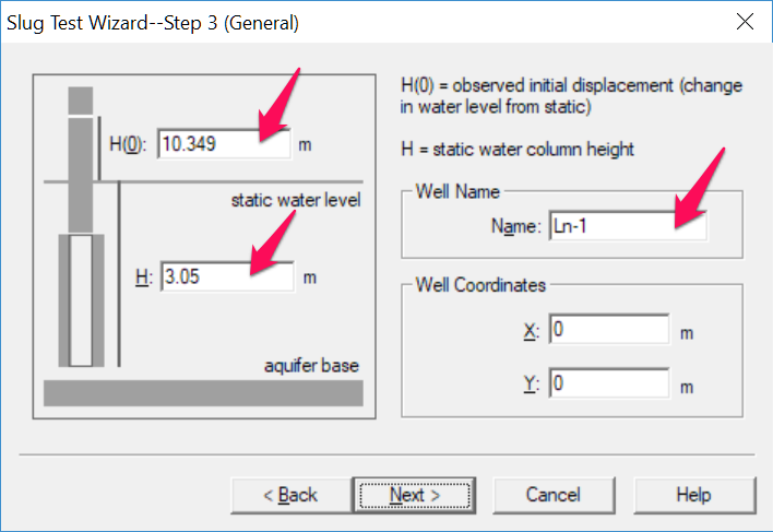
Data provided in Butler (1998) indicate the initial displacement, $H_0$, was 10.349 m. In addition, assume for the purpose of analysis a static water column height, $H$, equal to 3.05 m.

Water-level readings from this slug test are available in a .csv file in the form of elapsed time since test initiation in seconds and displacement in meters (Butler 1998, Table 5.2).

Field Data Inspection

At this stage, it's often convenient to use an application like Excel to make a quick plot of field water-level measurements for the purpose of identifying any transformations required to generate elapsed time since start of test and displacement. In this example, however, properly transformed elapsed time and displacement readings have been provided so you may inspect the data after entering them into AQTESOLV.

Data Entry

Begin your interpretation of the slug test data by creating a new AQTESOLV data set. In this example, you will use the Slug Test Wizard to facilitate data entry.

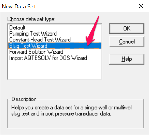
1. Start the AQTESOLV application (v. 4.0 and higher) and choose File > New to create a new data set that will contain data from the slug test. Select Slug Test Wizard to enter data from the slug test. Click OK.

   

2. The Slug Test Wizard prompts you for data required to analyze a slug test. Click Next to begin the wizard.
3. For the units of measurement, choose m for length, sec for time and m/day for hydraulic conductivity. Click Next.

   

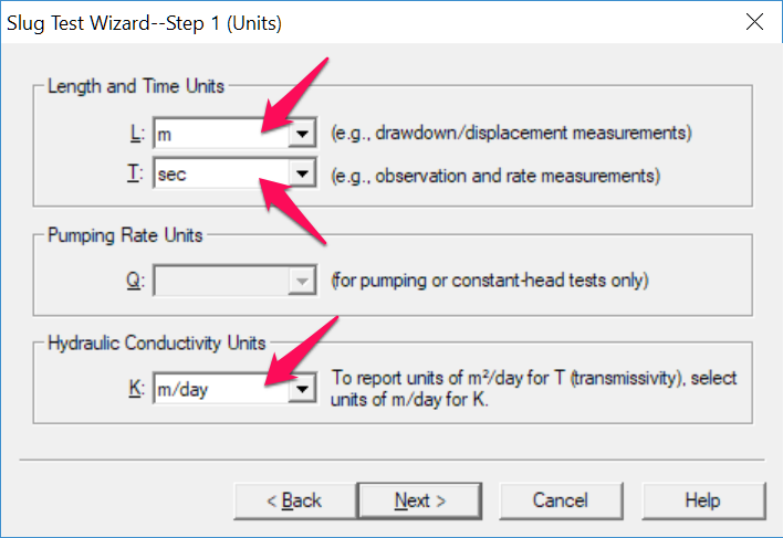
   The units of length and time should match the units of the elapsed time and displacement data that you will import from a data file. The length units also apply to well geometry data (e.g., screen length, casing radius, etc.) that you will enter into the data set.

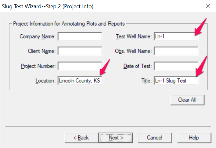
4. For project information, enter Lincoln County, KS for location, Ln-1 for test well name and Ln-1 Slug Test for title. Click Next.

   

5. For general test well data, enter 10.349 for initial displacement, 3.05 for static water column height and Ln-1 for well name. Enter coordinates of X=0 and Y=0. Click Next.

   

6. For aquifer data, enter 3.05 for aquifer thickness. Assume hydraulic conductivity is isotropic and enter 1 for anisotropy ratio. Click Next.

   

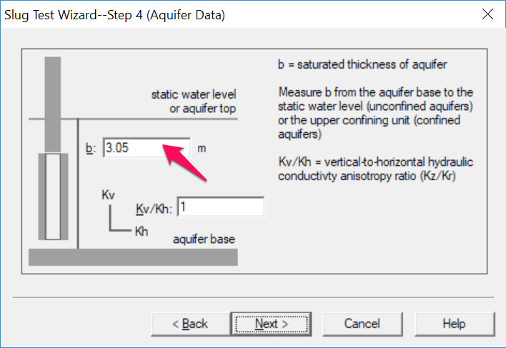
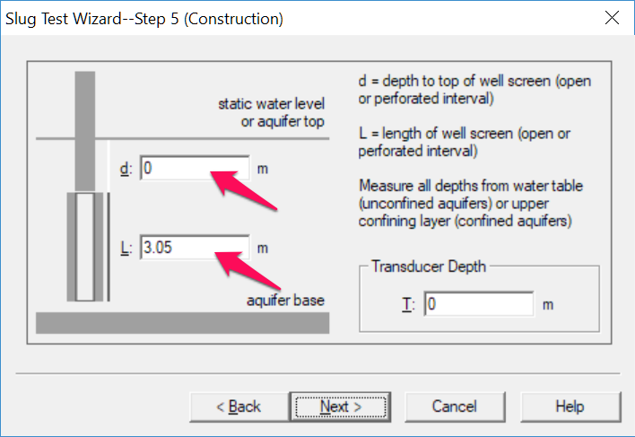
7. For construction data, enter 0 for depth to top of screen and 3.05 for screen length (a fully penetrating well). Assume the transducer measures the position of the water surface in the well and enter 0 for transducer depth. Click Next.

   

8. For radius data, enter 0.025 for casing radius and 0.071 for well radius. Assume no well skin and enter 0.071 for skin radius. Click Next.

   

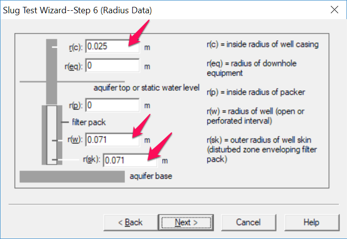
   In this instance, the filter pack is expected to be more permeable than the formation; hence, the effective well radius is taken as the borehole radius and not the screen radius.

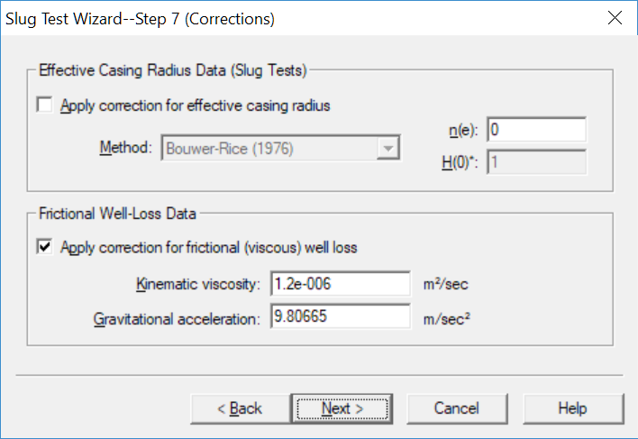
9. No corrections are needed for this test. The correction for effective casing radius only applies to wells screened across the water table. Click Next.

   

10. For observations, import data from the .csv file. Click Import to open the Import Wizard for observation data.

    

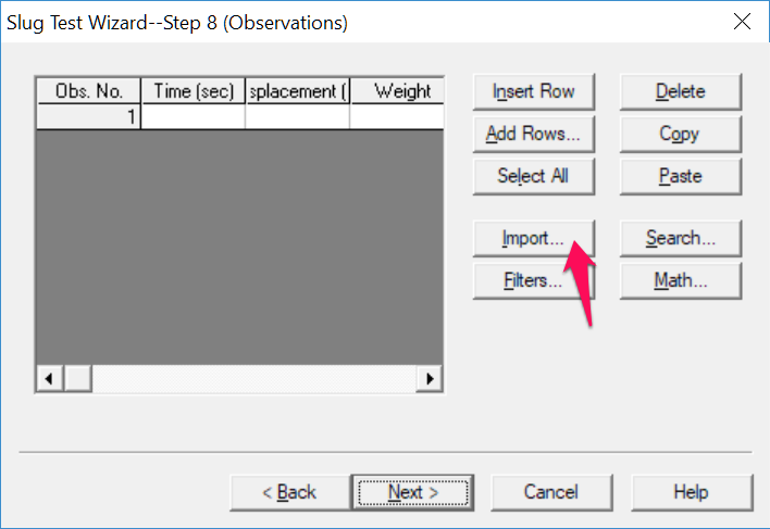
    In Step 1 of the Import Wizard, click Browse to select a file to import. Open the file Ln-1.csv containing the data from the test. Click Next to proceed to Step 2.

    

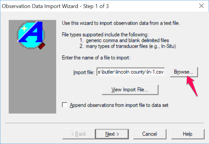
    In Step 2 of the Import Wizard, choose columns of data to import from the file. Enter 1 for the column containing elapsed time and 2 for the column containing displacement. Click Next to proceed to Step 3.

    

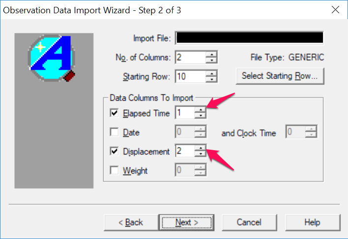
    In Step 3 of the Import Wizard, no transformations are needed as the import file already contains values of elapsed time since start of test and displacement. Click Finish to import the data from the file.

    

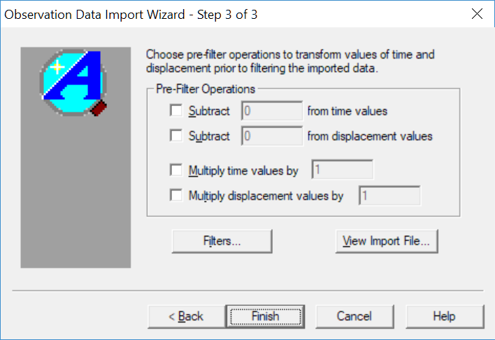
    Click OK when the Import Wizard has finished importing the file.

11. Click Next to complete the Slug Test Wizard.

    

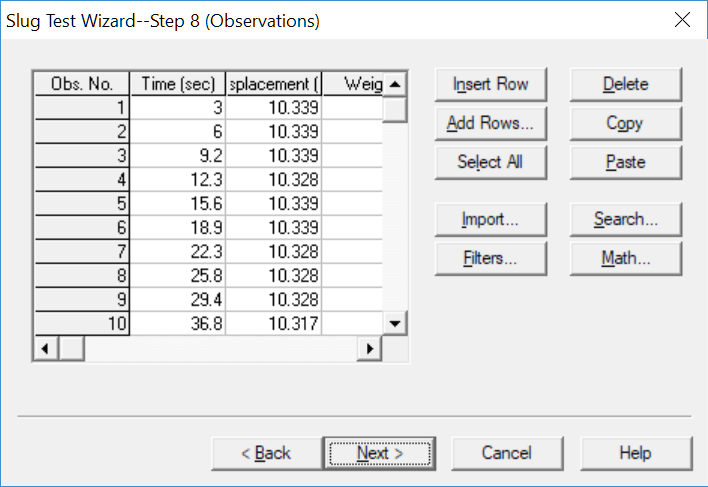
12. Click Finish after entering all of the data to finish the Slug Test Wizard.

Upon completion of the Slug Test Wizard, AQTESOLV automatically displays an Error Log that identifies errors in the data set. If the Error Log detects any mistakes, choose options from the Edit menu to correct them. In this example, the Error Log informs you that the initial displacement exceeds the aquifer thickness but you may ignore the warning because the aquifer is confined and the actual static water column height in the well exceeded the initial displacement.

At this point, it's a good idea to save your work. Save the data set by choosing Save As from the File menu. Choose a folder and enter Ln-1 for the name of the file. Click Save. AQTESOLV saves the file with an .aqt extension.

Match Solutions

You will now analyze the test data with the Cooper et al. (1967) solution for an overdamped slug test in a control well that fully penetrates a confined aquifer.

See Butler (1998, p. 59) for more information on the interpretation of this slug test with the Cooper et al. solution.

1. Choose Displacement-Time from the View menu to display a plot of the test data.

   Displacement is the change in water level in the well from its static (equilibrium) position.

2. Choose Log-Linear Axes from the View menu.

   Inspection of the data plot reveals an inverted sigmoidal curve that is typical of overdamped slug tests in low- to moderate-K aquifers.

3. Choose Options from the View menu. In the Plots tab, check Normalized head to display data as normalized head. Click OK.

   Normalized head is defined as displacement measured at elapsed time $t$ divided by initial displacement, $H_t/H_0$.

4. Choose Solution from the Match menu. Remove the check from Solution is inactive. Click the + next to Confined Aquifers to expand the list of available solutions for confined aquifers. Select Cooper-Bredehoeft-Papadopulos (1967) and click OK.
5. Choose Automatic from the Match menu and click Estimate to perform automatic curve matching with the Cooper et al. model.
6. When estimation is complete, click OK and then Close. Click OK to view the new position of the type curve.

   

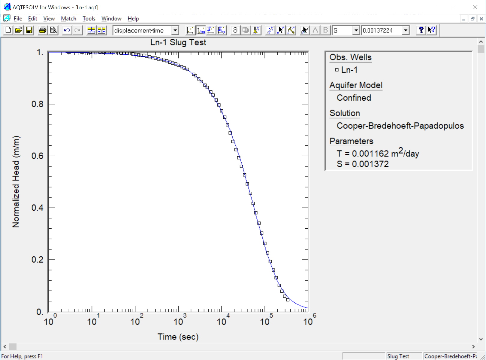
   The estimated value of $T$ = 0.001162 m²/day shown on the plot corresponds to $K$ = 0.00038 m/day. Butler (1998) reported a value of $K$ = 0.00037 m/day for these data.

   Choose Report from the View menu to find the value of $K$ when AQTESOLV estimates $T$ for the aquifer.

   AQTESOLV yielded an estimate of $S$ = 0.001372 which is a reasonable value for a confined aquifer. A nearly identical value of $S$ = 0.00134 was determined by Butler (1998).

7. Choose Save from the File menu to save your work.

Next you will use the quasi steady-state method of Hvorslev (1951) to estimate $K$ from the same set of data. The Hvorslev solution ignores formation storativity and allows you to match a straight line to response data. The result will serve as a check on our analysis with the Cooper et al. solution.

See Butler (1998, p. 69) for more information on the interpretation of this slug test with the Hvorslev method.

1. Choose Solution from the Match menu to select a method for analyzing the data.
2. From the available solutions for Confined Aquifers, select Hvorslev (1951) and click OK.

   With the Hvorslev solution, the plot legend shows two parameters: K (hydraulic conductivity) and y0 (intercept of the line on the y axis).

3. Choose Options from the View menu. In the Plots tab, check Recommended head range to display the range of normalized head recommended by Butler (1998) for matching the Hvorslev solution. Click OK.
4. Choose Visual from the Match menu to perform visual curve matching with the Hvorslev solution.
   • To perform visual matching, move the mouse to a point where you wish to begin drawing a new line.
   • Click and hold down the left mouse button to anchor the new line at this point.
   • Continue to hold the mouse button down and move the mouse to match a new straight line to your data. As you move the mouse, AQTESOLV draws a straight line between the anchor point and the position of the mouse.
   • Release the left mouse button when you have finished matching a new straight line. AQTESOLV automatically updates the plot legend to reflect changes in parameter values.
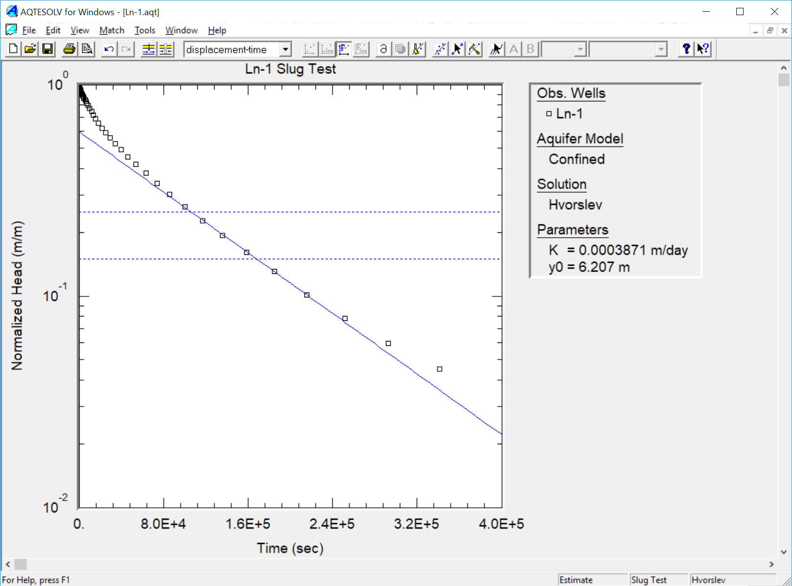
5. Repeat the previous step as needed to estimate $K$ by matching the straight line to the data within the recommended head range.

   

   The estimated $K$ = 0.0003871 from the Hvorslev analysis is very close to the value obtained with the Cooper et al. method.

   You could use automatic estimation to match the Hvorslev solution to these data; however, visual matching is generally more effective for matching straight-line solutions because you can apply your judgment to fit the line to the appropriate range of data.

6. Choose Save As from the File menu to save your new analysis. Enter Ln-1-Hvorslev for the name of the file. Click Save.

Finally you will apply the Peres et al. (1989) solution to estimate $T$ from the Ln-1 slug test. The Peres et al. method transforms data from a slug test into an equivalent constant-rate pumping test after which one may match a straight line to the transformed data. The result will provide an additional check on foregoing previous analyses.

Successful application of the Peres et al. (1989) deconvolution method is contingent upon (1) initiating a slug test with a relatively large $H_0$, (2) using a high-accuracy sensor and (3) extending the test to complete recovery (Butler 1998).

1. Choose Solution from the Match menu to select a method for analyzing the data.
2. From the available solutions for Confined Aquifers, select Peres et al. (1989) deconvolution and click OK.

   The Peres et al. solution plots equivalent drawdown (for a constant-rate pumping test) as a function of time on semi-logarithmic axes. For a slug test of sufficient duration and measurement accuracy, a straight line develops at late time that you can match with the Cooper and Jacob (1946) solution.

3. Choose Visual from the Match menu to perform visual curve matching with the Peres et al. solution.
   • To perform visual matching, move the mouse to a point where you wish to begin drawing a new line.
   • Click and hold down the left mouse button to anchor the new line at this point.
   • Continue to hold the mouse button down and move the mouse to match a new straight line to your data. As you move the mouse, AQTESOLV draws a straight line between the anchor point and the position of the mouse.
   • Release the left mouse button when you have finished matching a new straight line. AQTESOLV automatically updates the plot legend to reflect changes in parameter values.
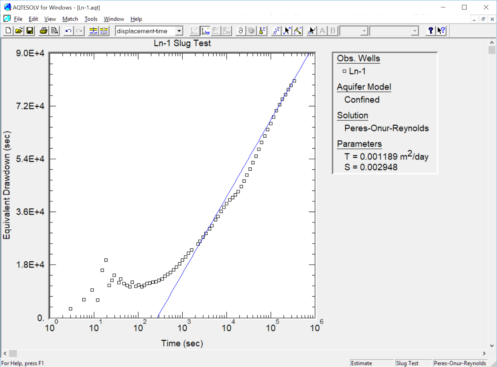
4. Repeat the previous step as needed to estimate $T$ by matching the straight line to late-time data.

   

   The estimated $T$ = 0.0001189 from the Peres et al. analysis is very close to the value obtained with the Cooper et al. method.

   You could use automatic estimation to match the Peres et al. solution to these data; however, visual matching is generally more effective for straight-line solutions because you can apply your judgment to fit the line to the appropriate range of data.

5. Choose Save As from the File menu to save your new analysis. Enter Ln-1-Peres for the name of the file. Click Save.

   For more information on the interpretation of this slug test with the Peres et al. solution, refer to Butler (1998, p. 77).