Derivative Analysis

Derivative analysis is powerful diagnostic tool that enhances the interpretation of data from pumping tests. Features difficult to discern in drawdown data alone are often readily apparent through the application of the derivative procedure. Groundwater hydrologists use derivative analysis to identify important flow regimes encountered during a pumping test, detect aquifer boundaries and select appropriate aquifer models.

Derivative analysis has its origins in the petroleum industry literature (Bourdet et al. 1983; Bourdet et al. 1989) and has been gaining attention among groundwater hydrologists for a number of years (Spane and Wurstner 1993; Renard et al. 2009).

The derivative used for pumping test interpretation is given by the slope of drawdown data plotted on a graph with semilog axes (linear drawdown and logarithmic time) as shown on the figure below.

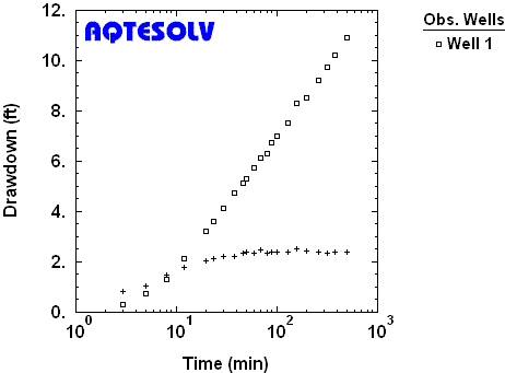
Note that the derivative reaches a plateau when the Cooper-Jacob straight line method would be appropriate for matching drawdown data to estimate aquifer properties in a nonleaky confined aquifer of infinite extent (infinite-acting radial flow).

The Bourdet derivative (Bourdet et al. 1989) uses the following simple three-point formula to compute derivatives from drawdown data by numerical differentiation:

$${\left(\frac{\partial s}{\partial \ln T}\right)}_{\text{i}}=\frac{\left(\Delta s_{\mathrm{i-1}}/\Delta \ln T_{\mathrm{i-1}}\right)\Delta \ln T_{\mathrm{i+1}}+\left(\Delta s_{\mathrm{i+1}}/\Delta \ln T_{\mathrm{i+1}}\right)\Delta \ln T_{\mathrm{i-1}}}{\Delta \ln T_{\mathrm{i-1}}+\Delta \ln T_{\mathrm{i+1}}}$$

where $s$ is drawdown and $T$ is an appropriate time function (e.g., elapsed time or Agarwal equivalent time). Essentially, this formula is a weighted average of slopes computed from data points on either side of data point $\text{i}$. In the above formula, the two slopes are

$$\Delta s_{\mathrm{i-1}}/\Delta \ln T_{\mathrm{i-1}}$$

and

$$\Delta s_{\mathrm{i+1}}/\Delta \ln T_{\mathrm{i+1}}$$

These slopes are also known as the left and right derivatives, respectively.

An important aspect of performing derivative analysis is the selection of an appropriate calculation method. Bourdet (2002) recommends using a nearest neighbor method (adjacent points) for preliminary derivative analysis; however, this method often results in noisy derivative data. To remove noise from calculated derivatives, the Bourdet method uses data points separated by a fixed distance measured in logarithmic time. Typically, the logarithmic separation or differentiation interval (L) required to remove noise ranges between 0.1 and 0.5 (Horne 1995); however, L values as large as 1.0 may be necessary for infrequently sampled data. In selecting the differentiation interval, one must exercise care to avoid overly smoothing the data.

Spane and Wurstner (1993) present an alternate method for computing derivatives. Like the Bourdet method, the Spane method uses a logarithmic differentiation interval; however, instead of using three points in the derivative computation, the Spane method computes the left and right derivatives by applying linear regression to all of the points falling within the differentiation interval. In some cases, one finds that the Spane method produces a smoother derivative than the Bourdet method.

End Effects

End effects occur when computing derivatives near the beginning or end of a set of drawdown data. For example, fewer data points are available for computing the right derivative near the end of a test. Bourdet et al. (1989) provide procedures for overcoming such computational limitations, but one often finds in practice that derivatives calculated near the end of a data set are less reliable (Horne 1995).

Application of Derivative Smoothing

Successful application of derivative analysis nearly always requires smoothing to remove noise from the calculated derivatives. The benefit of derivative smoothing is illustrated by the following example from a constant-rate pumping test in an unconfined aquifer (Kruseman and de Ridder 1994). Without smoothing, the derivative is noisy and yields little useful information. Application of smoothing produces a cleaner derivative signal that suggests delayed yield in an unconfined aquifer.

Derivative Plot Without Smoothing

Derivative Plot With Smoothing

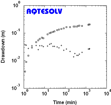
Plot of drawdown (squares) and derivative (crosses) from a piezometer monitored during a constant-rate pumping test in an unconfined aquifer (Kruseman and de Ridder 1994). The smoothed derivatives calculated with the Bourdet method suggest delayed yield. For this example, smoothing with the Spane method produces a similar derivative plot.

Derivative analysis is an invaluable tool for diagnosing of a number of distinct flow regimes. Examples of flow regimes that one may discern with derivative analysis include infinite-acting radial flow, wellbore storage, linear flow, bilinear flow, inter-porosity flow and boundaries.

To help identify flow regimes, it is convenient to classify them, in a broad sense, according to their time of occurrence during a constant-rate pumping test (early, intermediate or late). Of course, this classification is idealized and some of the features noted may not become apparent in a pumping test of short duration. Well locations and aquifer geometries also play a role in the chronology of flow regimes. For example, wells located near a river may not exhibit the derivative plateau associated with infinite-acting radial flow before a recharge boundary effect is observed.

Flow Regimes Classified by Time of Occurrence

Early Time Flow Regimes

• wellbore storage (confined aquifer)
• linear flow (vertical fracture)

Intermediate Time Flow Regimes

• infinite-acting radial flow (see most examples in catalog)
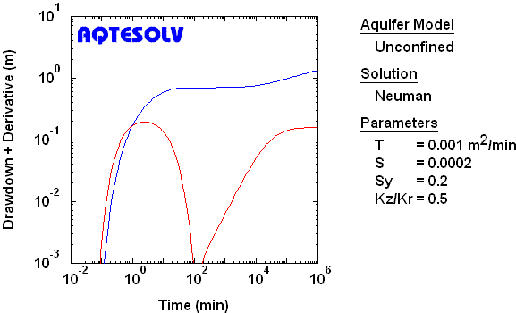
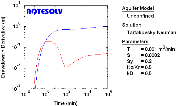
• delayed yield (delayed gravity response)
• inter-porosity flow (double porosity)
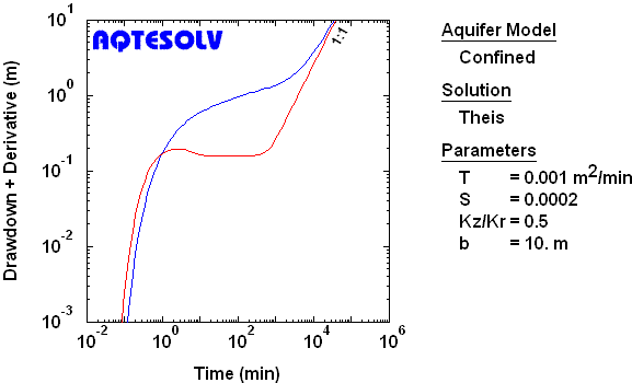
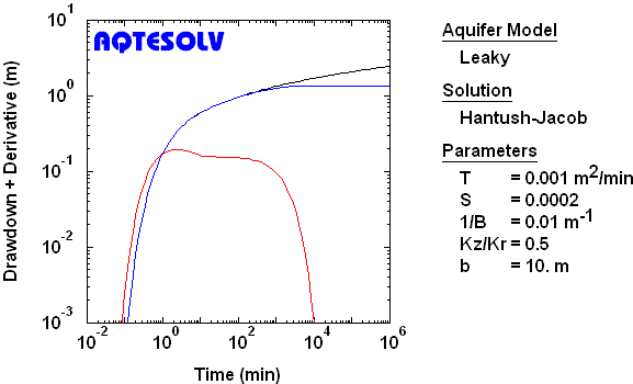
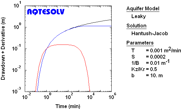
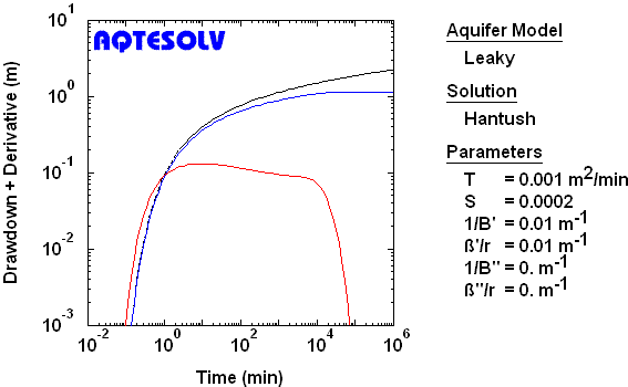
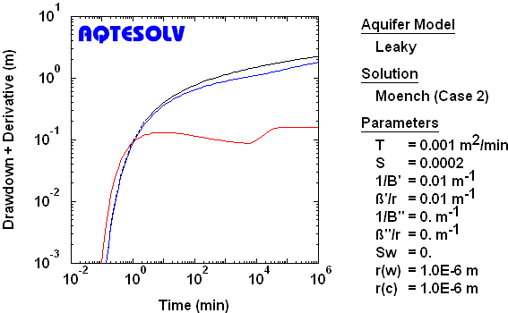
• leakage (incompressible aquitard, Case 1; compressible aquitard, Case 1; compressible aquitard, Case 2)
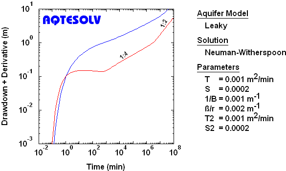
• bilinear flow (compressible aquitard, channel aquifer)

Late Time Flow Regimes

• infinite linear boundary (recharge boundary, barrier boundary)
• linear flow (channel aquifer)
• bilinear flow (channel aquifer with permeable boundaries)
• pseudo-steady-state flow (closed aquifer)

Summary of Flow Regime Characteristics

Flow Regime	Characteristic
infinite-acting radial flow	derivative plateau
wellbore storage	1:1 slope on log s vs log t
linear flow (1, 2, 3, 4)	1:2 slope on log s vs log t
bilinear flow (1, 2)	1:4 slope on log s vs log t
recharge boundary	drawdown plateau
barrier boundary	derivative plateaus separated by factor of two
pseudo-steady state flow	1:1 slope on log s vs log t

Derivative plots combine drawdown and derivative data on a single plot. The typical derivative plot used for diagnostic purposes is displayed on log-log axes. A catalog of derivative plots is invaluable to the practicing hydrogeologist by providing models (signatures) of drawdown and derivative responses for specific flow regimes and boundary conditions. The following catalog includes aquifer models and flow regimes not available in compilations by Spane and Wurstner (1993) and Renard et al. (2009).

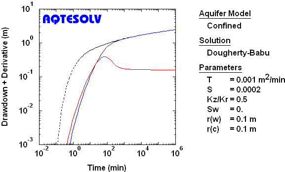
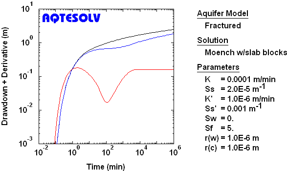
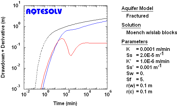
On the derivative plots presented below, drawdown and derivative responses are displayed as solid blue and red curves, respectively. For reference, the Theis solution is shown on selected plots by a dashed black curve. The following table provides well and aquifer parameters assumed for the plots (unless otherwise noted):

Pumping (Control) Well
constant discharge rate =	0.002 m3/min
casing radius =	0.1 m
well radius =	0.1 m
depth to top of screen =	5 m
screen length =	5 m
Piezometer
radial distance =	3.16 m
depth =	0.75 m
Aquifer
thickness =	10 m
vertical-to-horizontal anisotropy =	0.5

Nonleaky Confined Aquifer

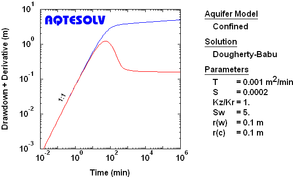
Finite-Diameter Source with Wellbore Storage

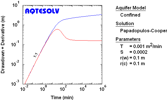
To identify wellbore storage in the control (pumped) well, look for coincident drawdown and derivative curves having a unit (1:1) slope at early time.

Observation Well, Line Source

Observation Well, Finite-Diameter Source with Wellbore Storage

Recharge Boundary

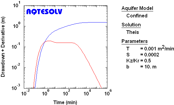
To identify a single infinite recharge (constant-head) boundary, look for a drawdown plateau and derivative curve plunging toward zero at late time. This behavior is similar to a leaky confined aquifer with an incompressible aquitard and constant-head source aquifer.

Barrier Boundary

To identify a single infinite barrier (no-flow) boundary, look for two derivative plateaus separated by a factor of two. On semi-log axes, the drawdown slope doubles.

Channel Aquifer

To identify linear flow in a channel (strip) aquifer, look for drawdown and derivative curves having a 1:2 slope and factor of two separation at late time.

Channel Aquifer with Permeable Boundaries

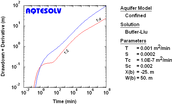
To identify linear flow in a channel (strip) aquifer with permeable boundaries, look for drawdown and derivative curves having a 1:2 slope and factor of two separation at intermediate time. To identify bilinear flow, look for drawdown and derivative curves having a 1:4 slope and factor of four separation at late time.

Closed Aquifer

To identify pseudo-steady state flow in a closed aquifer, look for coincident drawdown and derivative curves having a unit (1:1) slope at late time.

Leaky Confined Aquifer

Partial Penetration, Incompressible Aquitard, Case 1

Full Penetration, Incompressible Aquitard, Case 1

Full Penetration, Compressible Aquitard, Case 1

Full Penetration, Compressible Aquitard, Case 2

Full Penetration, Compressible Aquitard, Channel Aquifer

Unconfined Aquifer

Instantaneous Drainage at Water Table

Noninstantaneous Drainage at Water Table

Double-Porosity Aquifer with Fracture Skin

Line Source

Finite-Diameter Source

Vertical Fracture

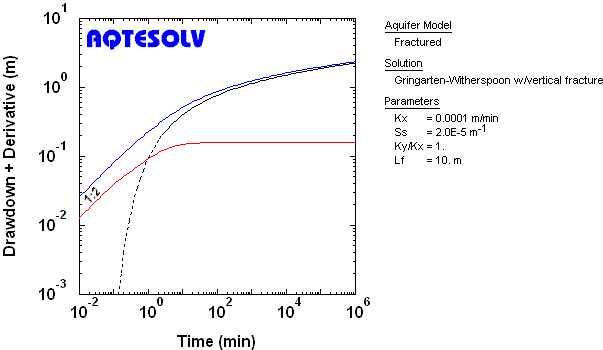
To identify linear flow to a well located along an infinite-conductivity vertical plane fracture, look for drawdown and derivative curves having a 1:2 slope and factor of two separation at early time.