AQTESOLV Tips
Follow
AQTESOLV
Follow AQTESOLV on LinkedIn!
How do I copy/paste transducer/datalogger data from a spreadsheet (e.g., Excel) into AQTESOLV?
How do I copy/paste an AQTESOLV plot into other software (e.g., PowerPoint)?
Can I export type curve data to a file?
How do I convert logger data from linear sampling to a logarithmic schedule?
- Choose Edit>Wells, select a well and click Modify.
- Click the Observations tab.
- Click Select All to filter all observations.
- Click Filters to view filter options.
- In the Time Filters, check the option for Retain change in log time >= minimum and enter a value of 0.05 (=1/20) to retain 20 measurements per log cycle time. To retain 10 data points per log cycle time, enter 0.10 (=1/10). Click OK.
- Click OK to proceed with the filtering operation.
- AQTESOLV displays the number of observations filtered and the number of observations retained. Click OK.
How do I generate contour plots of drawdown?
You may use Surfer to prepare contour plots of drawdown if you have the software installed on your computer. Choose View>Contour to launch the Grid Wizard which prompts you for information needed to create a grid (.grd) file for contouring. AQTESOLV will automatically launch Surfer and display the contour plot for you. A sample contour plot from a wellfield predictive simulation is shown below.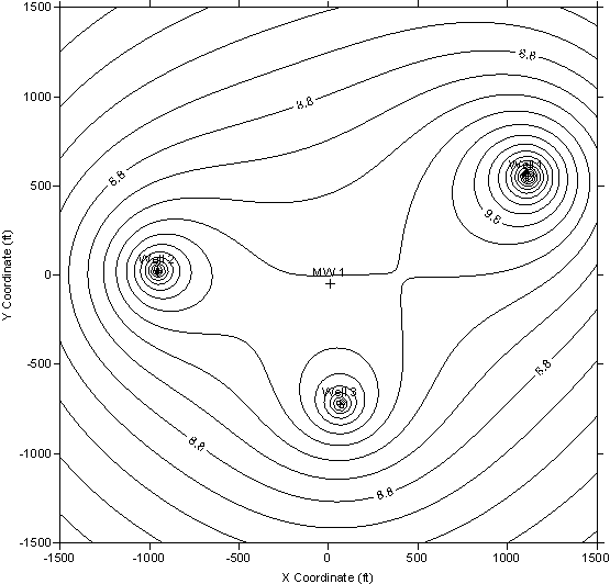
If you don't have Surfer, 3DField is an alternative program that you may download for free and use to prepare two-dimensional contour plots from grid files created by AQTESOLV.
What is the reference for entering well screen depths?
Enter well screen depths measured from the top of the aquifer not from land surface. In a confined aquifer, measure depths from the upper confining unit. In an unconfined aquifer, measure depths from the static water table. For a well screened across the water table, click here.
My well is screened across the water table. What do I enter for d (depth to top of screen) and L (screen length)?
For a well screened across the water table, enter d=0. Enter the submerged length of screen for L. Ignore any portion of the screen above the water table.
Can I manually enter/edit aquifer properties like T and S?
Choose Match>Toolbox and click the Parameters tab to enter aquifer properties for the active solution. Edit properties in the Value column of the spreadsheet.
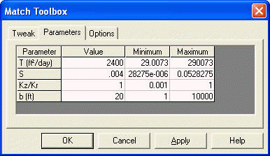
Tip: The Minimum and Maximum columns in the spreadsheet allow you to control the parameter range used in the Tweak tab.
How do I enter the pumping rate for a constant-rate pumping test?
When you enter rates into AQTESOLV, enter the time for each measured rate as the elapsed time since the start of the test when the rate becomes active. Thus, for a constant-rate test, enter zero for time and the constant rate into the rates spreadsheet. You only need to enter one pumping rate for a constant-rate test.
For example, if you are analyzing drawdown data from a pumping test performed at a constant-rate of 100 gpm, you only need to enter the following row in the rates spreadsheet for the pumping well:
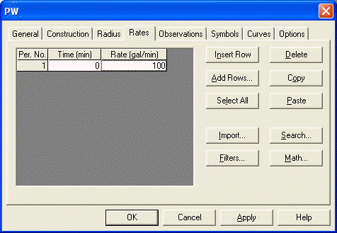
Tip: There is no need to enter a pumping rate corresponding to each drawdown measurement you collect.
What's the best way to learn how to use AQTESOLV?
Choose Help>Contents and Index to open the Help file installed with AQTESOLV. In the Contents tab of the Help file, open the Quick Start chapter and navigate to the Examples topic. You will find many detailed tutorials with step-by-step instructions explaining how to use the software for the interpretation of data from pumping tests, slug tests and constant-head tests.
Find additional online tutorials in Examples section of the AQTESOLV web site.
How do I modify, add or remove wells?
Choose Edit>Wells to edit wells in your data set. Select a well in the list and click Modify to make changes to the well or Delete to remove it from the data set. Click New to add a new well to your data set.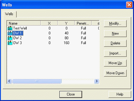
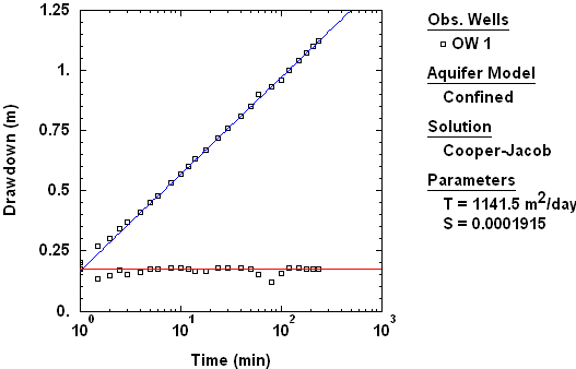
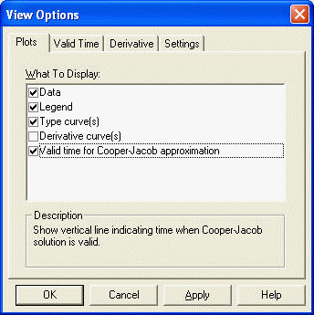
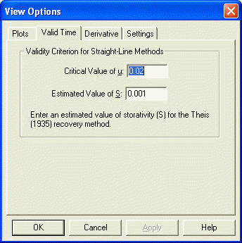
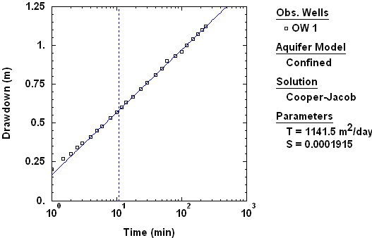
How do I check the validity of a match with the Cooper and Jacob (1946) straight-line method?
In AQTESOLV, you have two options for checking when the Cooper and Jacob solution is valid:
- Choose View>Options>Plots tab and check the option to display Valid time for Cooper-Jacob approximation.
In the Valid Time tab, you may assign the critical value of u (default = 0.01).
AQTESOLV displays a vertical dashed line on your data plot to indicate the time when the Cooper and Jacob solution is valid. Note that the position of the line depends on the values of T (transmissivity) and S (storage coefficient) for the line that you've matched.
- In the Pro version of AQTESOLV, you may use derivative analysis (View>Options) to identify when the drawdown data have a constant slope on a semilog plot. A derivative plateau (= constant slope) indicates a period where you could match the Cooper and Jacob solution and estimate T of the aquifer assuming the underlying assumptions of the solution, such as infinite-acting aquifer conditions, are met.