Theis Recovery Solution for Nonleaky Confined Aquifers

Charles Vernon Theis (1900-1987) was the first groundwater hydrologist to develop a rigorous mathematical model of transient flow of water to a pumping well by recognizing the physical analogy between heat flow in solids and groundwater flow in porous media.

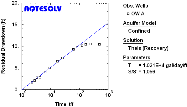
The Theis (1935) solution is useful for determining the transmissivity of nonleaky confined aquifers from recovery tests. Analysis involves matching a straight line to residual drawdown data collected after the termination of a pumping test. The solution assumes a line source for the pumped well and therefore neglects wellbore storage.

If your observation data contain both pumping and recovery measurements, you may use the Theis recovery method to analyze just the recovery data.

Assumptions

• aquifer has infinite areal extent
• aquifer is homogeneous, isotropic and of uniform thickness
• control well is fully penetrating
• flow to control well is horizontal
• aquifer is nonleaky confined
• flow is unsteady
• water is released instantaneously from storage with decline of hydraulic head
• diameter of pumping well is very small so that storage in the well can be neglected
• values of $u^{\prime }$ are small (i.e., $r$ is small and $t^{\prime }$ is large)

Equations

C.V. Theis, a groundwater hydrologist with the U.S. Geological Survey, derived the following approximate linear equation to predict residual drawdown in a homogeneous, isotropic and nonleaky confined aquifer assuming a fully penetrating line sink that discharged at a constant rate prior to recovery:

$$s^{\prime }=\frac{2.303Q}{4\pi T}\left[\log \left(\frac{t}{t^{\prime }}\right)-\log \left(\frac{S}{S^{\prime }}\right)\right]\text{(1)}$$

where

• $Q$ is pumping rate [L³/T]
• $s^{\prime }$ is residual drawdown [L]
• $S$ is storativity during pumping [dimensionless]
• $S^{\prime }$ is storativity during recovery [dimensionless]
• $t$ is elapsed time since start of pumping [T]
• $t^{\prime }$ is elapsed time since pumping stopped [T]
• $T$ is transmissivity [L²/T]

To apply the Theis recovery method given by (1), plot $s^{\prime }$ as a function of $\log (t/t^{\prime })$ on semi-logarithmic axes and draw a straight line through the data (example). Determine $T$ using the following equation:

$$T=\frac{2.303Q}{4\pi \mathrm{\Delta }{s}^{\prime }}\text{(2)}$$

where

• $\mathrm{\Delta }{s}^{\prime }$ is the slope of the fitted line (change in residual drawdown per log cycle equivalent time)

$S/S^{\prime }$ is found from the intersection of the line with the $\log (t/t^{\prime })$ axis of the plot. In the absence of boundary effects, $S/S^{\prime }$ should be close to unity. A value of $S/S^{\prime }>1$ suggests recharge during the test; whereas $S/S^{\prime }<1$ may indicate a no-flow boundary.

Variable-Rate Pumping

For uninterrupted variable-rate pumping, one may use the principle of superposition in time to compute residual drawdown for $N$ constant-rate steps (Birsoy and Summers (1980)):

$$s^{\prime }=\frac{\text{2.303}{Q}_N}{4\pi T}\text{log}\left(\frac{\text{2.25}T}{r^{2}S}{\beta }_{t^{\prime }}\right)\text{(3)}$$ $${\beta }_{t^{\prime }}=\prod _{n=1}^N{\left(\frac{t-t_n}{t^{\prime }}\right)}^{\Delta Q_n/Q_N}\text{(4)}$$ $$\Delta Q_n=Q_n-Q_{n-1}\text{(5)}$$

where

• ${\beta }_{t^{\prime }}$ is adjusted time [T]
• $Q_n$ is pumping rate in the $n^{\mathrm{th}}$ constant-rate step [L³/T]
• $Q_N$ is pumping rate in the last constant-rate step prior to recovery [L³/T]
• $s^{\prime }$ is residual drawdown [L]
• $t_n$ is elapsed time when the $n^{\mathrm{th}}$ constant-rate step starts [T]

Data Requirements

• pumping and observation well locations
• pumping rate(s)
• observation well measurements (time and displacement)

Solution Options

• variable pumping rates

Estimated Parameters

AQTESOLV provides visual and automatic methods for matching the Theis recovery method to recovery test data. The estimated aquifer properties are as follows:

• $T$ (transmissivity)
• $S/S^{\prime }$ (ratio of storativity during pumping to storativity during recovery)

Curve Matching Tips

• Choose Match>Visual to perform visual curve matching using the procedure for straight-line solutions.
• Use parameter tweaking to perform visual curve matching and sensitivity analysis.
• Perform visual curve matching prior to automatic estimation to obtain reasonable starting values for the aquifer properties.

Benchmark

References

Theis, C.V., 1935. The relation between the lowering of the piezometric surface and the rate and duration of discharge of a well using groundwater storage, Am. Geophys. Union Trans., vol. 16, pp. 519-524.